This chapter describes the steps to load and analyze data, when working with Mobile Mapping data in eCognition. Mobile mapping data is geospatial data that is collected from a mobile vehicle or platform, e.g. Trimbles MX series. The data consists of images, so called time frames, captured in viewing direction of a camera and point cloud data in addition.
Loading Mobile Mapping Data
Create a new workspace.
Load data to a new project (Import data or new project):
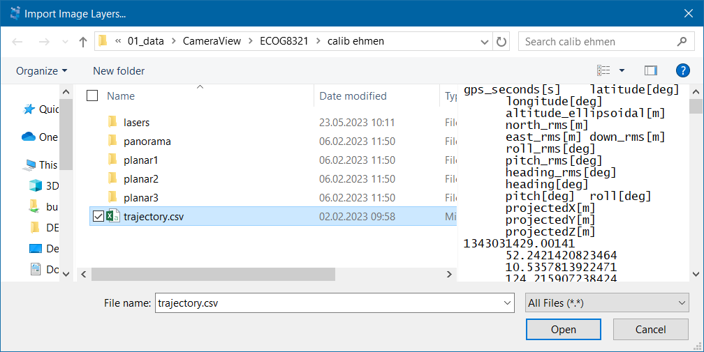
In the import image layer dialog select the trajectory.csv and click Open to load the TMX® data structure (export from Trimble Business Center).
Example: ...\Project Data\trajectory.csv
Now the Import Mobile Mapping Data dialog opens:
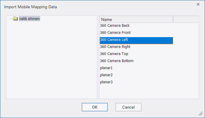
If you select the folder on the left side you see the contents displayed on the right side.
Select one of the Camera positions (e.g. 360 Camera Left) > Click OK.
In the Create Project dialog the image layers and point cloud files (*.las files) are now added.
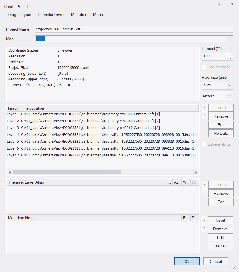
In the same dialog you can now add additional point clouds layers that belong to the loaded data or remove layers that are not needed for the analysis. To add layers:
- select Insert image layer in the Create Project dialog
- select the point clouds layers *.las file(s) that belong to your image data and click Open
Finally, in the Create Project dialog select OK to open the new project.
Tip - You can also see details of the loaded data in the View > Source View dialog and load the files needed in this dialog using drag and drop, alternatively you can use File > Modify open project.
Image Layers
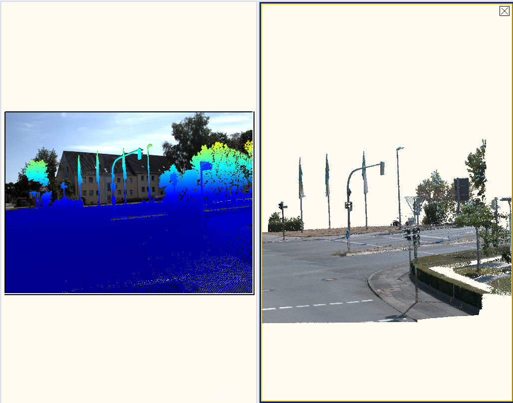
The first three image layers represent the captured image data in viewing direction of the camera position you selected.
Point Clouds
Visualize the point clouds by activating the check box in this section of the view settings dialog. With one point cloud active a 3D view can be opened via the 3D toolbar. The 3D view also reflects the position of the time frame animation. (Note that regions cannot be visualized in the 3D view for mobile mapping data).
The point clouds layers are displayed per default in height rendering mode. You can change this in the View Settings lower pane > Point clouds > Point cloud settings > Render mode > e.g. RGB
Time Series Toolbar
To navigate between the image layers hold the Ctrl button and scroll with the wheel of your mouse forward (and backwards).
Alternatively you can select the frames directly using the Time series toolbar that opens automatically when loading mobile mapping data. If not opened by default the toolbar can be opened in View > Toolbars > Time Series:
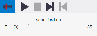
Frame Navigation: Use this slider to navigate through the frames by selecting a frame position.
Start/Stop time frame animation - shows the time frames in a loop until you press stop (Ctrl + Space)
Show next time frame - shows the next time frame starting from this position (Ctrl + Mouse Wheel zoom in or Ctrl + Right)
Show prev time frame - show the previous time frame (Ctrl + Mouse Wheel zoom out or Ctrl + Left)
The current frame number is displayed in the bottom right corner of the map view - time frame 2 corresponds to T: 2.
Working with Mobile Mapping Data
When working with Mobile Mapping data you can use the following approach:
- To open the point cloud data in the 3D view in the view settings click the 3D button (alternatively select View > Toolbars > 3D) and then select the Full 3D data extent button . For mobile mapping data the full subset is opened immediately. (How to navigate in 3D data see next chapter How to navigate in the 3D window).
- Additional raster or point cloud layers can be generated using the algorithms Rasterize point cloud
 or Create temporary point cloud
  (see
(see - When rasterizing a point cloud, gaps within the data can be interpolated using the Kernel parameter of the rasterize point cloud algorithm or based on created image objects.
- Classification:
Point cloud points can be classified using eCognitions point cloud classification algorithms, e.g. Assign class to point cloud . Features are available e.g. in Feature view > Point cloud features.
Alternatively the image layers can be classified using the standard classification algorithms (classification , assign class
  ). For this approach the features based on '2D objects' are available in Feature view > Object features > Point cloud. In a last step the classification result can then be assigned back to the point cloud using algorithm assign class to point cloud .
 - Finally, results can be exported using one of the export algorithms or the export point cloud algorithm
 .
.
How to navigate in the 3D window
- Left Mouse Button (LMB): While holding down the LMB you can move the mouse up (zoom out) and down (zoom in) to achieve a smooth zooming. This zooming corresponds directly to mouse movement. The cursor turns to a double-pointed arrow.
- Left Mouse Button (LMB): With the Object Information window open and point cloud features selected in the Feature view - a single click on a point cloud point shows feature values for the selected point that is visualized as a big red dot. (To change the color go to View > Display mode > Edit highlight colors > Selection color.) When you select a point in the 3D view the same point is highlighted in the main window and vice-versa.
- Right Mouse Button (RMB): While holding down, RMB is used for rotating the point cloud around a center point located in the middle of the selected subset. The cursor turns to a circular arrow and the center point of the subset appears.
Right Mouse Button (RMB) - with activated custom center of rotation : While holding down, RMB is used for rotating the point cloud, now with the center of rotation located at the position where this right mouse button was activated.
 - Mouse Wheel: Rotating the wheel produces a discrete zoom. This zooming is performed in individual steps, corresponding to the rotation of the wheel. The cursor turns to a double-pointed arrow.
- Both LMB and RMB / Press Mouse Wheel: Holding down both the left and right mouse buttons or pressing the mouse wheel enables the user to pan in 3D space. The cursor turns to a hand.
- Alternatively, from the toolbar you can also select the Panning button or the Zoom Out Center and Zoom In Center buttons.
 Zoom Scene to Window button: helps you to reset the observer position, all zoom and rotation steps to default.
